
“Has the Fed Been a Failure?” is Chapter 8 of Money Free and Unfree (2017), by George Selgin. It originally appeared as a paper in the Journal of Macroeconomics 34, no. 3 (September 2012), by Selgin, William D. Lastrapes and Lawrence White. It has a few notions that I think are worth mentioning here. Also, it is relatively recent, and updates current discussion on these topics.
One of the more useful sections of the paper is “Volatility of Output and Unemployment,” which takes up the question of how accurate the standard (Kuznetz-Kendrick) estimates of pre-1914 economic cycles are.
Christina Romer’s (1986a, 1989, 2000) influential work has, however, cast doubt even on this more attenuated claim. According to her, the Kuznets-Kendrick pre-1929 real GNP estimates overstate the volatility of the pre-Fed output relative to that of later periods, in part because they are based on fewer component series than later estimates and because they conflate nominal and real values, but mainly because the real component series are almost exclusively for commodities, the output of which is generally much more volatile than that of other kinds of output. From 1947 to 1985, for example, commodity output as a whole was about two and a third times more volatile than real GNP. (p.223.)
The Romer estimate of percentage standard deviation from trend for 1869-1914 was 2.664, vs. 5.064 for the standard. That is a lot different. In general, I don’t take estimates of GDP and “prices” from before 1914 very seriously, because just as is described, they are based on rather skimpy data, including estimates of “price levels” that are highly correlated to commodity prices. As I’ve noted, commodity prices in the post-1971 era are about twice as volatile as commodity prices during gold standard eras, but “prices” (CPI) are much more stable, basically because it has totally different characteristics. Also, there is also the simple question of economic structure. The U.S. economy was simply more commodity-based in those days than it is now. Thus, it might have had more ups and downs related to somewhat volatile commodity prices. This has nothing to do with monetary issues, but is simply a reflection of the economy of that time. Today, emerging market countries typically have higher levels of volatility of various CPI indices, simply because commodities (energy and food) make up more of the typical CPI basket. This is just a matter of economic structure.
February 19, 2017: “Prices” and Value
March 3, 2016: The Myth of “Price Instability” During the Gold Standard Era
Second, the U.S. was not on a gold standard from 1861 to 1879, and indeed suffered a number of economic ups and downs which included a monetary component.
Also, there was quite a lot of turmoil and difficulty in the 1890s, due to three factors: 1) the Barings crisis of 1890, 2) The Panic of 1893, related to the threat of a devaluation of the dollar from “bimetallists,” and 3) The Panic of 1896, also related to the threat of dollar devaluation, finally resolved in the victory of pro-gold William McKinley in the 1896 presidential election. Once you remove these factors, the 1880-1914 period looks rather good indeed.
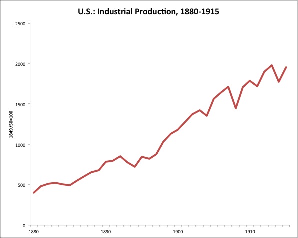
You can see here the turmoil in the 1890s, related to the bimetallist threat as I mentioned. There’s also a minor dip in 1904 (possibly related to the San Francisco earthquake that year, which had financial consequences in the East as well), the Panic of 1907, and of course the outbreak of World War I in 1914.
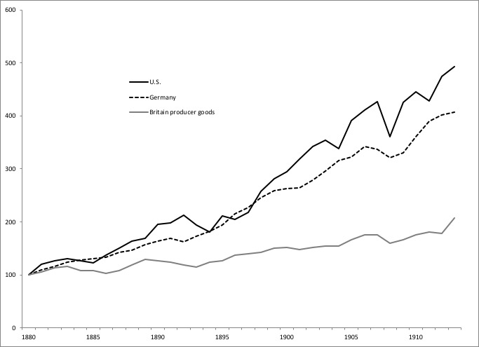
There was no meaningful decline in industrial production in Germany, which was also of course on gold but didn’t have the currency-devaluation issues, so you can’t blame that on gold.
Complementary revisions of historical unemployment data by Romer (1986b) and J. R. Vernon (1994) … likewise suggest that the post-1948 stabilization of unemployment apparent in Stanley Lebergott’s (1964) standard series is an artifact of the data. (p. 224)
… Albrecht Ritschl and colleagues (2008) employ “dynamic factor analysis” to uncover a latent common factor capturing the comovements in 53 time series that have been consistently reported since 1867. According to their benchmark model … they find that post-World War II volatility was a third greater than pre-Fed volatility. (p. 226)
Measuring “volatility” alone, over such time periods, does not amount to much in my opinion. You have to have some historical understanding of what was going on at the time, which of course does not lend itself very well to statistics. Nevertheless, the message again is that there was a lot less “volatility” during that time than people often think.
John Keating and John Nye (1998) … find that aggregate supply shocks were of overwhelming importance in the earlier period, accounting for 95 percent of real output’s … variance at all horizons. (p. 226-7)
“Aggregate demand and supply shocks” amount to what I would call: nonmonetary factors. Now we have some academics saying that 95% of all volatility during the pre-1914 era was due to nonmonetary factors. This is good, since you can’t claim that 95% of “volatility” is due to nonmonetary factors, and then blame the gold standard. However, I would not agree with this. As I mentioned, most of the problems of that era can be traced to monetary factors, primarily the floating dollar before 1879, and the “free coinage”(dollar devaluation) issues in the 1890s, which led to a lot of financial turmoil. (The 1890 Barings crisis itself was related to the devaluation of the Argentine peso in the face of sovereign default.)
A more recent study by Michael Bordo and Angela Redish (2004) … [found that] aggregate supply shocks accounted for 89 percent of pre-Fed output variance at a 1-year horizon and 80 percent of such variance after 10 years. (p. 227)
We [the authors] find that aggregate supply shocks account for between 81 percent and 86 percent of the … variance of pre-Fed output up to a three-year horizon, as opposed to less than 42 percent of the variance after World War II. (p. 228)
Thus, “variance” (economic ups and downs) was 81%-86% “nonmonetary” in the pre-Fed era, and only 42% “nonmonetary” after WWII, according to these estimates.
The NBER’s chronology [of business cycles] has nonetheless been faulted for seriously exaggerating both the frequency and the duration of pre-Fed cycles and, thereby, exaggerating the Fed’s contribution to economic stability. According to Romer (1994: 575), whereas the NBER’s post-1927 cycle reference dates are derived using data in levels, those for before 1927 are based on detrended data. This difference alone, Romer notes, results in a systematic overstatement of both the frequency and the duration of early contractions compared to modern ones. .. Romer arrives at a new set of reference dates that “radically alter one’s view of changes in the duration of contractions and expansions over time” … According to this new chronology, although contractions were indeed somewhat more frequent before the Fed’s establishment than after World War II … they were also almost three months shorter on average, and no more severe. Recoveries were also faster … (p. 234)
People living at the time thought the economy was doing rather well. It turns out that they were not wrong. On the subject of banking panics (related to the “lender of last resort” function, and seasonal variation in base money demand):
Bordo (1986) reports that, among half a dozen western countries he surveyed (the others being the United Kingdom, Sweden, Germany, France and Canada), the United States alone experienced banking crises. (p. 239-240)
Thus, these issues have nothing to do with gold’s usefulness as a stable standard of value (or, variation in gold’s value that might cause financial problems), but rather, nonmonetary country-specific factors.
Dismissals of the gold standard as a viable policy option have often been based on flawed assessments of its past performance … The instability in the U.S. financial system during the pre-Fed period was due to serious flaws in the U.S. bank regulatory system rather than the gold standard. (p. 253)
A second indictment of the gold standard derives from fear of secular deflation. We noted above the importance of distinguishing benign from harmful deflation, while also observing that the secular deflation that characterized much of the classical gold standard period was benign, accompanying vigorous real growth. It is true that spokesmen for the interests of farmers complained about secular deflation. They appear to have believed, mistakenly, that overall deflation was lowering their real or relative incomes, as though nominal rather than the real factors were lowering the prices of what they sold relative to the prices of what they bought. Or they were seeking a bit of unexpected inflation to reduce, ex post, the real value of the debts they had incurred in farm mechanization. Their complaints reflected misperception or special-interest pleading rather than any genuine harm being done by a benign deflation (Beckworth 2007).
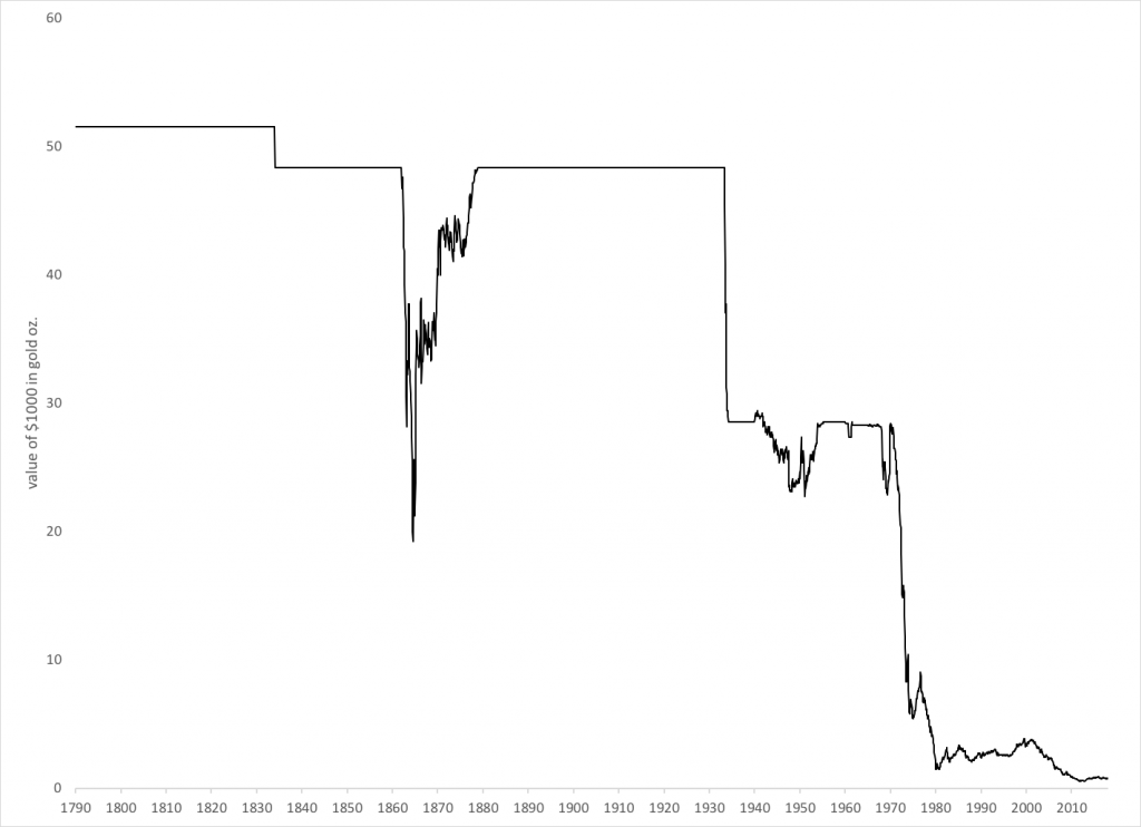
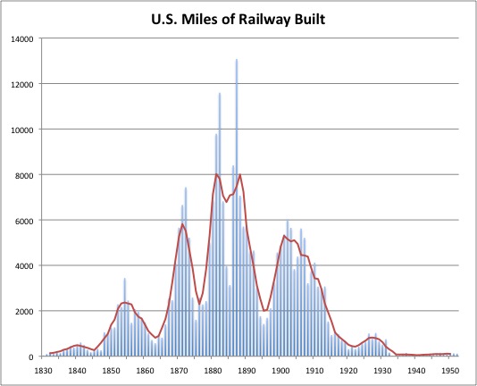
This refers to the decline in commodity prices, especially 1880-1896. The economy was actually doing quite well at the time — the rate of increase in industrial production 1880-1896 (the period of declining commodity prices) was nearly the same as 1896-1914 (rising commodity prices), both periods among the best in U.S. history. I’ve shown that there was an enormous increase in commodity production in the U.S. and worldwide during this time, due in part to the enormous expansion of railways and steamships, which allowed vast tracts of land to be opened for agriculture and mining for the world market, not only in the U.S. but also places like Argentina, Brazil, Australia, Canada, South Africa, India, China and Eastern Europe.
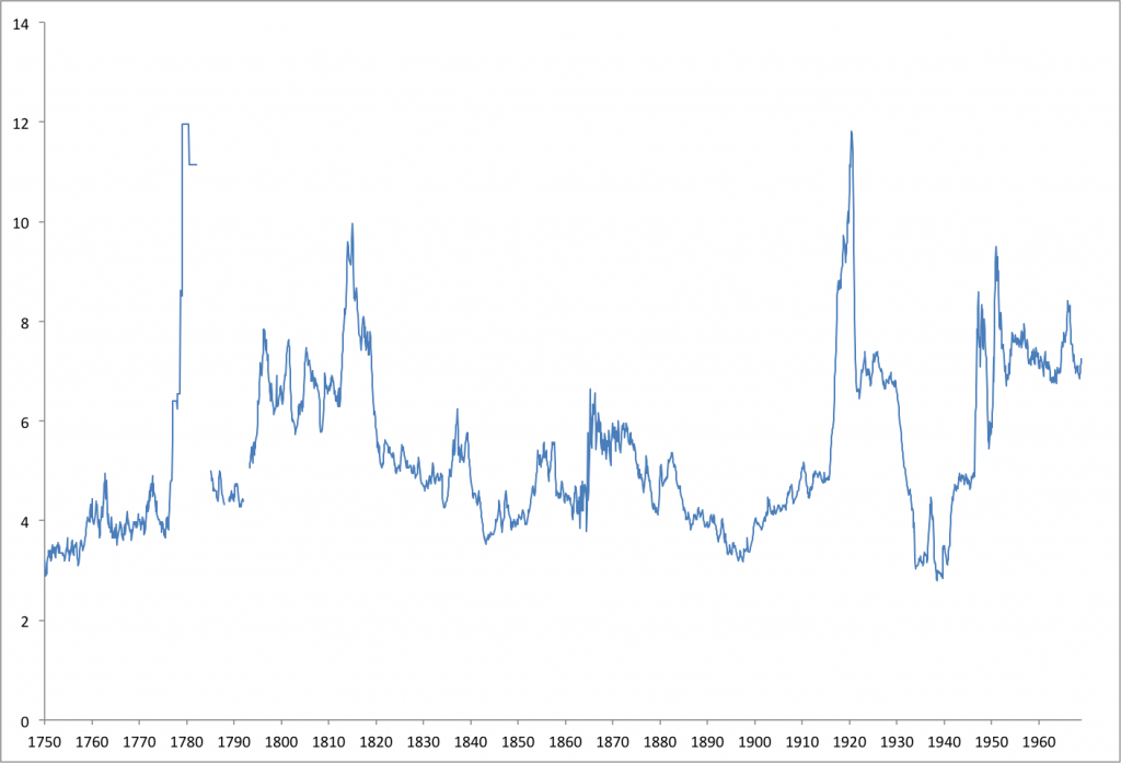
U.S.: Warren-Pearson commodity price index in gold oz., 1750-1970
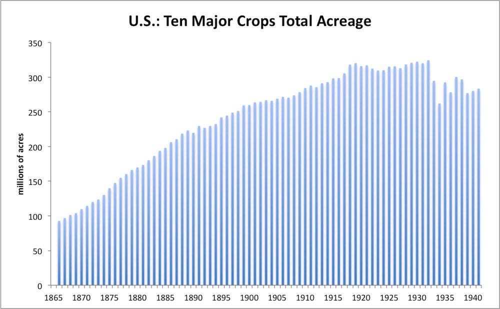
We can see here the huge increase in total acreage planted in the U.S. between 1870 and 1900, coinciding with the great railway expansion. The increase is about 150%. All that land had to be bought, planted and developed, of course, which probably meant that farmers had a lot of debt, and might have been in a lot of trouble when selling prices were not as high as they had planned. After 1900, the rate of increase backs off considerably (in percentage growth rate terms), and the level in 1940 is hardly different than 1900. Not surprisingly, from 1920-1970 (excepting the Great Depression), when the economy was doing well but commodity production was rather restrained, commodity prices vs. gold were at rather high levels.
In general, when commodity prices fall and production is increasing, the decline in price is due to an excess of supply vs. demand. When commodity prices fall and production is stagnant or falling, the decline in price is due to a decline in demand vs. supply. The decline in prices in the 1880-1896 period was mostly the former — although the financial turmoil of the 1890s also introduced a suppression of demand, as we can see from the stagnation of industrial production during that time (industrial production being, of course, the “demand” for commodities). Thus, we should not at all assume that the decline in commodity prices during that time was a matter of a change in gold’s monetary value. The authors here argue that it was primarily — perhaps, entirely — a nonmonetary effect.
All in all, a fine showing, with many points relevant to our interests here.
