The 1890s
February 26, 2012
The 1890s are another time that the Keynesian economists like to point to as an example of “gold rising in value.” What they mean by that is, that commodity prices were falling. For several years leading up to the 1896 presidential election, the Democratic party made various threats to effectively devalue the dollar by allowing “free coinage of silver.” This alone caused quite a lot of financial turmoil and distress, as you might expect when a government starts to tell people that they will devalue the currency. However, on top of that, the decline in commodity prices itself was crushing many farmers, who were often in debt.
February 12, 2012: The Warren Pearson Index
Here’s what it looks like:
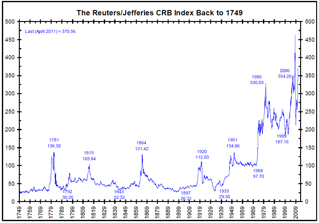
What do we see here?
There is a big peak in commodities prices in 1864, related of course to the Civil War. The dollar was devalued during this time, which of course had the corresponding effect on commodities prices. On top of that, you have the usual supply/demand characteristics of war, which is increased demand (for war materials), combined with decreased supply, because the farmers are in the battlefield shooting each other instead of growing crops.
The decline in commodity prices from 1864 to 1879 corresponds to the re-valuation of the dollar, the return of its value to the prewar gold parity, which was accomplished in 1879. From there comes a little more of a decline into 1897, and then a modest rebound in prices in the 1900-1913 period.
The 1870s and 1880s were the great decades of railway expansion in the United States. This allowed farmers who had really served just their local area — because you can’t really carry a bulk crop like corn for more than about twenty miles in a horse-drawn cart — to grow crops for long-distance trade. People bought land, borrowing money in the process, expecting to be able to put their crops on the train and sell it in New York or Charleston, and thenceforth to Europe or wherever. A flood of agricultural products hit the market, driving down prices, and thus bankrupting the farmers. This bad experience suppressed the expansion of farmland acreage beginning around 1900. A simple supply and demand story.
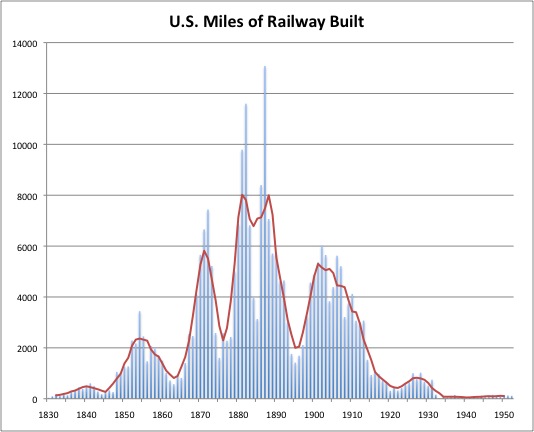
This is really incredible. The U.S. was adding 6000-8000 miles a year of railway track. This was all done with hand tools! The population of the U.S. in 1880 was 49 million people.
Imagine! Forty-nine million people, using hand tools, without electricity or petroleum, could lay six to eight thousand miles of rail track a year. China today is aiming for about 7,000 miles of rail track a year for the next ten years. This is with twenty-four times the population, using power tools and heavy equipment.
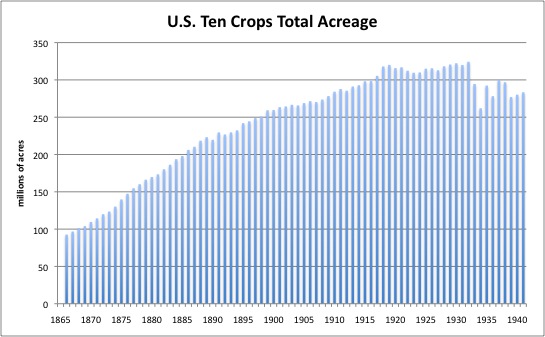
This shows the acreage under cultivation for the top ten commercial crops. See how it grows from 92.7 to 259.6, a 180% increase, in the 34 years from 1866 to 1900. However, from 1900 to 1940, forty years, it grows from 259.6 to 280.2, an increase of only 7.9%.
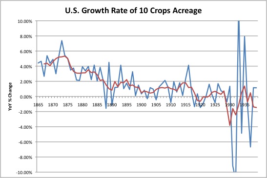
Here are YoY % Change figures, and a five-year moving average. We see that the growth rate in the 1870s and 1880s was in the realm of 3%-5% per year. This falls to about 1.5% per year in the 1890s and less than that after 1900.
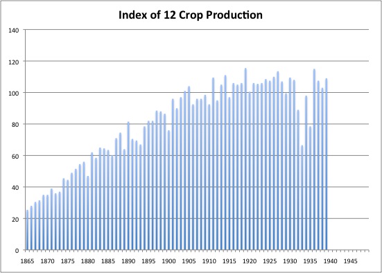
This index of production for the top 12 crops has a lot of variability due to the weather and so forth. The period 1910-1914=100 on this index. It goes from 25.5 in 1866 to 86.5 in 1900, an increase of 239% in 34 years. Then, from 1900 to 1940, it rises 26% in forty years.
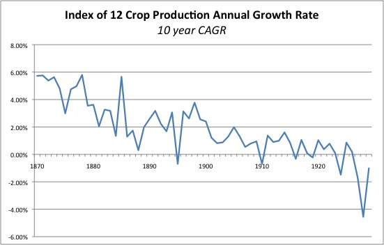
Here I am applying quite a lot of smoothing to the yearly growth rates. This is the compound annual growth rate for a ten year period centering on the indicated year. We can see that the average was around 5% in the 1870s, 3% in the 1880s and 1890s, and then it falls below 2% after 1900. Less supply = better prices.
In the 1890s, and then in the 1930s, people argued that you needed to devalue the currency to maintain “stable prices.” What they really meant was: declining commodity prices were hurting farmers, and causing them to default on their loans. Of course a devaluation would tend to support nominal commodity prices, and allow farmers to pay back their loans in a devalued currency. Note how much commodity prices rose in the 1940s. Did any of these “stable prices” advocates suggest that the dollar be returned to its $20.67/ounce pre-1933 parity? Of course not. Their “stable prices” arguments only go one way.
The market served its function in the 1890s. By removing any incentive to increase acreage under cultivation and farm output, the supply glut was resolved, and prices rebounded in the 1900-1910 decade. In the 1896 presidential election, the voters chose William McKinley, who promised to stay with the gold standard. Despite the difficulties of the 1890s, it worked out fine: the 1900-1914 period was a wonderful time of economic expansion in the U.S. and indeed throughout the world, the last hurrah of 19th Century Capitalism before the turmoil of the two world wars.
The information for these graphs comes from the NBER Macro History Database, a free online resource.
http://www.nber.org/data

