
Since we have been talking about “inflation” a lot recently, I thought I would bring up some points on that topic that have become more relevant. Even among the better monetary thinkers, there are a lot of funny ideas that are not quite true.
“Stable Money” does not produce a stable CPI. Over the longer term, commodity prices have had some stability under a gold standard, with a lot of shorter-term variation. This is exactly what you would expect if gold was perfectly stable in value. Gold is not perfectly stable, of course, but the observable variation in commodity prices does not serve as a counterexample to the proposition that gold’s stability is pretty good.
However, today’s CPI doesn’t have much relation to commodity prices. What we have seen is that the CPI, as it is commonly calculated by statistical agencies in the US and other countries, tends to rise in times of strong economic growth, even when the currency is stable in value.
May 22, 2019: How To Get Outrageous Growth Without “Inflation”
July 26, 2019: Stable Value Is Our Monetary Goal, Not “Stable Prices”
Thus, we cannot expect a Stable Money regime to produce “stable prices” (unchanging CPI). Maybe prices will go up, or down, for all kinds of reasons — not having to do with the value of the currency, which we have assumed as Stable. As I noted in those items, the CPI in Japan rose 70% during the 1960s, even while the yen was pegged to gold and commodity prices were dead flat. This was basically the result of high growth in Japan in those years. If you were hoping the gold standard would produce a flat CPI, you would have been disappointed. Hong Kong in the early 1990s had an even higher CPI, over 9% per annum, while the HKD was linked to the USD with a currency board. Others argue that perhaps the general price level would fall, due to increasing productivity, or competition from cheap foreign labor, or what have you. So, there might also be an extended period of price declines, again even with an idealized Stable Money system. In other words, there is a wide variety of nonmonetary factors that could influence the CPI, perhaps in a big way.
Focus on the Value of the currency, not Quantity
If we look at the history of writing about monetary topics, and experience in these matters, we find first that much of it occurred during the era of coinage (before paper money), from the seventh century BC to about 1650. Governments would often reduce the bullion content of their coins, diluting them with base metals. This was a sort of “currency devaluation.” The gold coin that once contained 10 grams of gold now contained 5 grams. Often, governments would do this by literally taking some gold coins (perhaps from tax revenue, or a debt issuance), melting them down and adding base metals, and then minting a larger number of new coins. Or, they would get the gold from government-owned mines, and make more coins out of the gold than they did in the past. So, the process of reducing the value of the coinage was inherently linked to the process of increasing the quantity of coinage, which was inherently linked to government finance.
So, for many centuries, we have had an explanation of “inflation” that usually has something to do with an increasing quantity of money linked with government spending. But, the “inflation” didn’t really come from the increasing quantity, but from the decreased value, which reflected the metal content of the coins. For example, let’s say a government purchased a metric ton of gold bullion from miners, financing this with debt, and then minted this into coins and spent it. The quantity of coins has increased, but their metal content is unchanged. The government spent the new coins. But, the new coins have the same amount of gold in them as the old. In this case, there would be no “monetary inflation” effect, although there would be some effects from the borrowing and spending.
A little afterward, beginning in the late 17th century, governments began to issue paper currencies. Again, the pattern was an increase in the quantity of money, linked to government spending, that resulted in a decline in the market value of the paper currency, and “monetary inflation.” This became particularly relevant during and after World War I, when nearly every major government engaged in printing press finance, including the United States, Britain and France. Of course, Germany and Austria took it the farthest, after the War, ending up in a terrible hyperinflation. This was a big influence on the Austrian writers including Ludwig von Mises.
This history gave rise to the popularity of the “equation of exchange,” often expressed as:
MV=PQ
This is: “money” X “velocity of money” = “Prices” X “Real Output”
In contemporary terms, “Prices” would be the GDP deflator (similar to CPI), and “Real Output” would be “Real GDP.” PQ thus equals nominal GDP.
This “equation” is mathematically correct, but also irrelevant. It is basically a tautology. It is equally true and correct that:
WV=PQ
Where: “Number of Winnebagos sold” X “Velocity of Winnebagos” = “Nominal GDP”
“Velocity” has no real external existence. It is merely the ratio between, in this case, Winnebagos and GDP.
As you can see, “money” (or Winnebagos) might go up, down or whatever, and NGDP might go up, down or whatever, and this equation will be true, but irrelevant. It is a tautology.
To reiterate, there is no informational content in this equation. It is a tautology. You could just as well say:
Google Hits for “Dua Lipa” * Velocity of “Dua Lipa” = Number of bicycles in China * The temperature at the South Pole
This is mathematically true, but meaningless.
However, “MV=PQ” is taken as an expression of the general idea that the growth of “money” will be proportional to “PQ” or NGDP. In other words, a rise in P (prices) is proportional to the degree that the growth of M exceeds the growth of Q. This is the “inflation,” and it is entirely monetary, since obviously we have no place in our equation for anything that is not monetary. Since the government is entirely responsible for “M” today (via central banks), it seems like the only way to get a rising P is with excessive M (assuming V is stable), and thus all “inflation” (rising P) is due to excessive M. It seems like there is “too much money (M) chasing too few goods (Q, or Real GDP).” It is a sort of expression of the coinage debasement and government paper money printing episodes of the pre-1930 era. But how to we explain, here, that the CPI in Japan rose 70% in a decade due entirely to growth effects, with no change in the value of the yen (vs. gold)? We cannot. It appears to be a matter of “MV” since that is the only thing on the other side of “PQ.”
Misinterpretation of this largely meaningless tautology soon leads to all kinds of funny notions that aren’t so. Note that there is no mention of the currency’s value here. We have the part about the government minting coins, but left out the part where the metal content of the coins is less than the old.
For example, we could have an argument that “a decrease in the number of hits for Dua Lipa must necessarily result in either a decrease in the number of bicycles in China, or a decrease in the temperature of the South Pole, assuming that Velocity is stable.” This is true. And then, when it turns out that Dua Lipa became less popular without much affecting bicycles or temperature, we then say: “But, there was a change in velocity!” Riiiiight.
In the sixteen years I have been writing on this website, I have never found need to refer to “MV=PQ” except to occasionally poke fun at those who take it seriously.
While these sorts of government money-printing episodes do take place, what we have seen during the twentieth century, and especially after the floating fiat period began in 1971, is a rather large disconnect between Quantity and Value. There is no question that Quantity affects Value, but the relationship is rather chaotic and complicated. Many episodes of monetary inflation have taken place without meaningful expansion of the money supply (quantity), or any direct relation with government spending. The value of the currency declines, but quantity stays the same, or perhaps the growth rate of quantity stays the same.
I have many examples of what I mean in my books. Here are a few:
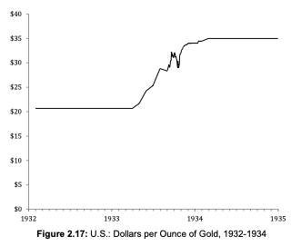
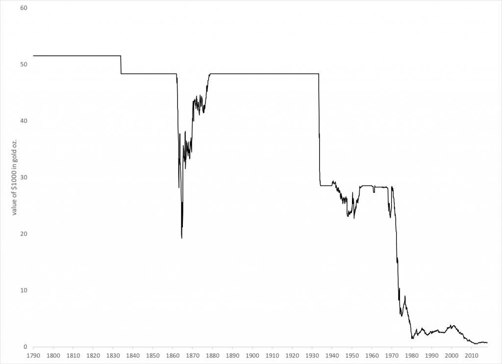
Here is the value of the US dollar, during the devaluation in 1933. The value fell, from $20.67/oz. to $35/oz. (it took more dollars to buy an ounce of gold = less value per dollar).
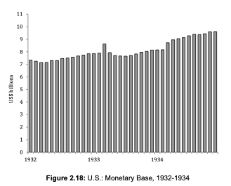
Here is the monetary base. It was dead flat during this devaluation episode. There was no increase in “M.” Just a decline in the value of the currency. This produced the desired inflationary effect, just as was planned by the Roosevelt Administration.
This inflationary effect was spread out over many years. Prices adjusted to the new value of the dollar, but it took a long time. I think a lot of it came in 1946-1950, in other words about 15 years after the 1933 devaluation, when the lifting of wartime price controls allowed the CPI to rise by quite a bit. Then, during the 1950s and 1960s, growth and prosperity also tended to push up prices, as measured by the CPI. The CPI rose a lot after 1934.
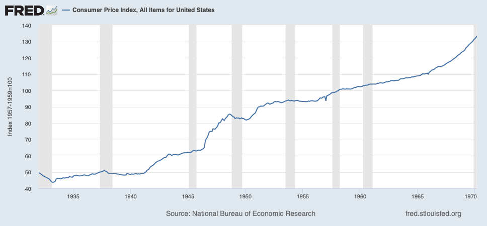
However, the value of the currency didn’t change. It was pegged at $35/oz. There was some considerable deviation from this ideal during WWII, and again at the end of the 1960s, but mostly it really was Stable at $35/oz.
In the meantime, the monetary base increased by huge amounts.
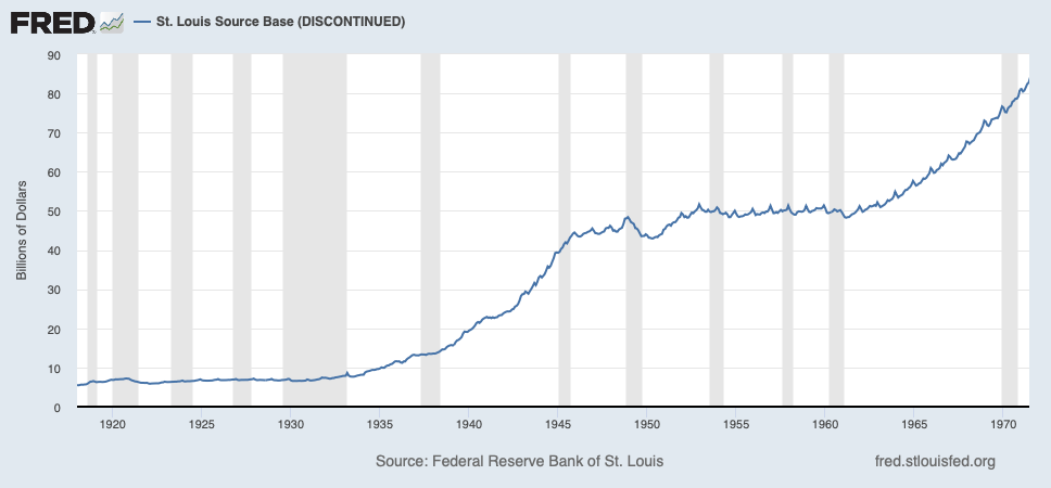
So, we have rising prices (CPI), and also a huge increase in “money,” but no decline in the value of the currency, which was basically at $35/oz. We had a change in value in 1933, but no change in the quantity, and then a huge change in the quantity in 1934-1970, and also a huge rise in the CPI, with no change in the value.
Note also that the price effects from the 1933 devaluation flowed through the economy over a period of years and decades. It was the devaluation (decline in value) that produced the “inflationary” effect. But, in the equation MV=PQ, there is no way to account for this time lag effect. Everything is in the present. It is present M and V and present PQ. In the present, the dollar was linked to gold at $35/oz. There was no problem there.
Value of the dollar vs. gold, including the WWII “softness.”
Another example comes from the 1970s. The dollar lost a huge amount of value, as expressed in the decline of its value vs. gold during that decade. This produced the “inflation” of that time.
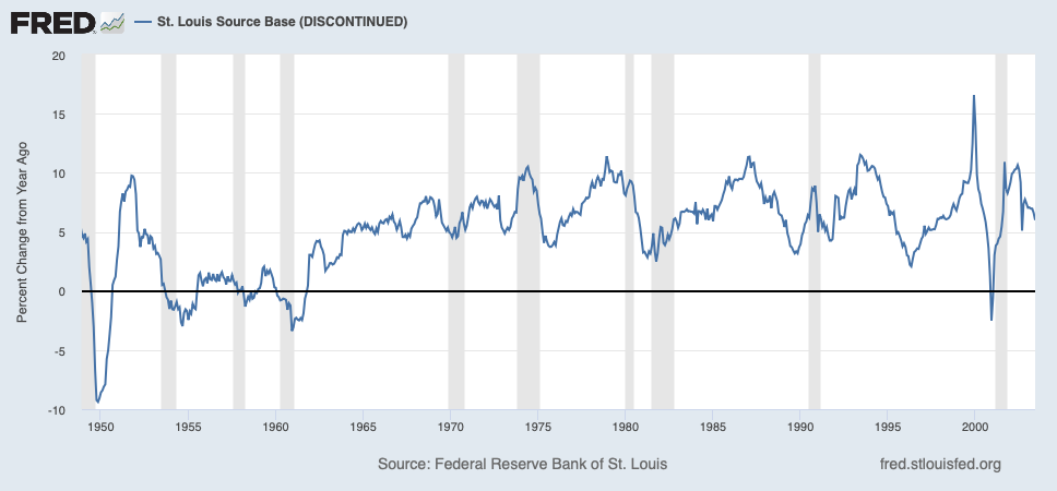
Here is the growth rate of the monetary base. It is hard to make much distinction here between the gold standard era of the 1960s, the wildly inflationary 1970s, or the disinflationary 1980s and 1990s. They all look about the same. If you were looking for some dramatic increase in the supply of money, perhaps linked to government spending, and this then flowing into NGDP via MV=PQ, you won’t find it here. You have to look at the value of the currency.
I think that if the dollar had remained linked to gold at $35/oz., and the economy had remained strong as it was in the 1960s, and there had been the Reagan tax cuts in the 1980s allowing even more growth but with the dollar remaining linked to gold at $35/oz. throughout, the growth rate of the monetary base would probably look rather similar.
While an increase in the quantity of money, perhaps linked to government spending, can certainly result in a decline in currency value, there is no “monetary inflation” unless there is a change in the value of the currency. However, this change in value can come about from a variety of situations — these are rather chaotic floating fiat currencies — including what you could call a “loss of confidence” or a “loss of faith,” which amounts to a huge change in currency value arising from a change in the mental state of investors, not M or V or P or Q, or something of that sort. Also, you can have huge changes in the quantity of money, as we have had since 2009 (for good reasons), and not too much change in the value. You can also have huge changes in prices (the CPI), with no change in the value of the currency.
Focus on the value.
