
Of the various “monetary aggregates” (at one point, I think over thirteen were identified), “M2” is perhaps the most commonly referenced. It is supposedly important. But why? To answer that, we have to first figure out what it is.
For many decades, “monetarism” has been waved in people’s faces as the proper way of understanding money. But, Monetarism has always been a floating-fiat construct of economic manipulation. Basically, it conflates “money” (the circulating medium), with “credit” (a process of financing economic activity, via contracts denominated in money), and through this, the economy as a whole. The contemporary version of Monetarism is NGDP Targeting (also known as “Market Monetarism“) which, as should be obvious to anyone, attempts an overarching total control of the economy, hitting a prescribed NGDP target, via monetary manipulation alone.
All of this is anathema to the Stable Value principles that most countries have always used. In the past, before 1971, the core of this “stable value” idea was the gold standard system — linking the value of currencies to gold. Today, most countries in the world do much the same thing by linking to the USD or EUR. In doing so, they must give up all ambitions to manage the domestic economy (perhaps by aiming at a specific NGDP), via some sort of currency manipulation.
The idea of a currency of Stable Value is similar to other standardized weights and measures. An ideal currency is a sort of constant of commerce. This is actually inherent in what “money” is. If this constant of commerce remains constant — of stable value — then there is no particular monetary problem, although there may be many other non-monetary problems. With a currency of stable value, an economy might crash into disaster, as the US economy did in 1929-1932, with nominal GDP falling 20%+. Or, an economy might enjoy a period of breathtaking growth, as Japan did in the 1960s, with nominal GDP rising 15%+ per year. Obviously, “stabilizing nominal GDP” is not a goal, although that is often one of the pleasant effects that take place when you do not disrupt economic processes by attempted macroeconomic manipulation that results in changing currency value.
Monetarist-flavored economists pay a lot of attention to various quantity statistics, particularly “M2.” These are not really monetary, but basically, measures of banking system activity. It is not very surprising that banking system activity tends to have an effect on, or is correlated with, the economy as a whole, or Nominal GDP. After all, the banking system is a big part of the economy. It is like saying that the distance of a person’s outstretched arms is about equal to their height. Very high correlation, not much useful causality. Nevertheless, there is an element of causality as well: bank lending, either expansion or contraction, tends to lead economic activity. You have to borrow the money before you spend it. Or, if you have to pay your loans back, but are unable to do any new borrowing (this is what “contraction” means), then you have less money to spend. This is not only directly related to economic activity, but also, price indexes. A contracting economy tends to have falling prices; an expanding economy often has rising prices. (This is the basic Keynesian “aggregate supply/aggregate demand” framework.) But, this also has a relationship to real monetary effects. A weak economy lacks “pricing power,” or “demand,” and so, price adjustments to changes in monetary value can be delayed or suppressed. A strong economy allows pricing changes to move through more quickly.
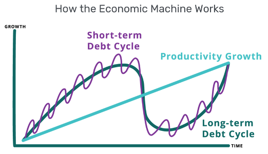
Around the middle of the twentieth century, from the 1920s to the 1960s, this sort of “credit cycle” analysis of recessions was more common. We don’t seem to hear much of this today. Probably, there are specialists who have focused on these topics — Lakshman Achuthan of the Economic Cycle Research Institute comes to mind. Also, it is a core element of Ray Dalio’s “How the Economic Machine Works” model.
First: “M2” is claimed to be a monetary measure, but it is really a measure of banks’ balance sheets. Basically, it is bank deposits, and currency in circulation. It does not include bank reserve balances at the Federal Reserve, a component of base money.
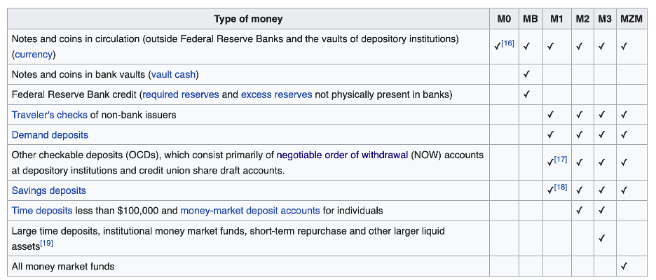
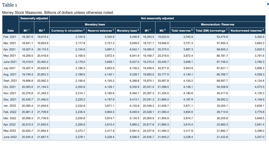
Since Currency in Circulation is about $2,278 billion, and M2 is about $21,645 billion, about 90% of M2 is bank deposits. Perhaps more than half of “currency in circulation” is actually outside the United States.
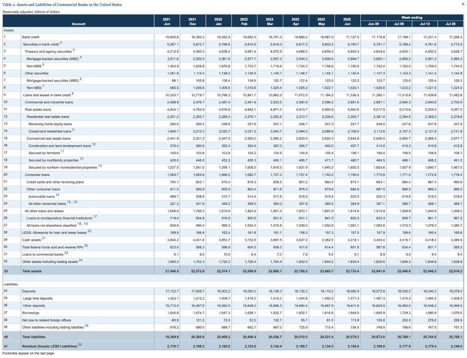
Deposits account for about 80% of bank liabilities and equity. The rest consists of a little bit of “other borrowings” (such as bonds), and bank capital, all of which tends to maintain stable proportions. Since balance sheets must balance, this means that Deposits (and thus M2) are basically a straight mirror image of Assets, which are lending and securities.
This does not really tell you anything about monetary conditions. For example, here is M2 in Greece:
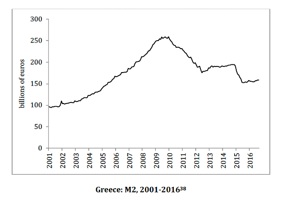
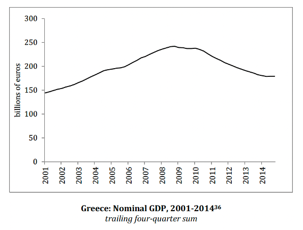
We see a huge contraction in M2 in Greece. This was not monetary, since Greece was using the euro at the time, and the euro wasn’t doing anything particularly odd. However, just as we should expect, this measure of the size of banks’ balance sheets (a giant contraction) was highly correlated to nominal GDP in Greece. Nominal GDP in Greece contracted by about 25%, which is a catastrophic, Great Depression-like figure.
For an example of how M2, NGDP and genuine monetary inflation can interact, an interesting example is presented by the 1930s and 1940s. Here is basically M2:
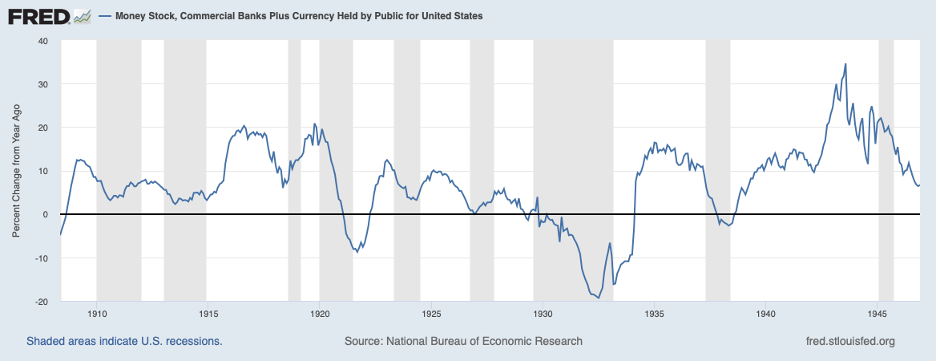
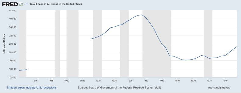
We see a dramatic contraction in the early 1930s. This was actually not monetary, but instead very similar to what happened in Greece. The actual “money supply” (the monetary base) was increasing at the time. There was no “monetary contraction,” but there was a large credit contraction. Bank lending stayed stagnant until WWII.
Also, we see a huge expansion in the 1940s, during the wartime boom. This was matched by a huge expansion in the monetary base, which is common in wartime.
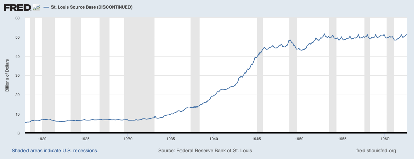
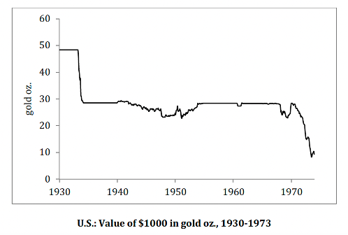
This monetary base expansion was conducted in the context of a rather lax, almost floating currency compared to the $35/oz. official gold parity. However, the deviation from $35/oz. was not so much (reaching a nadir of about $43/oz.), and the USD returned to $35/oz. more precisely after the war, in the early 1950s.
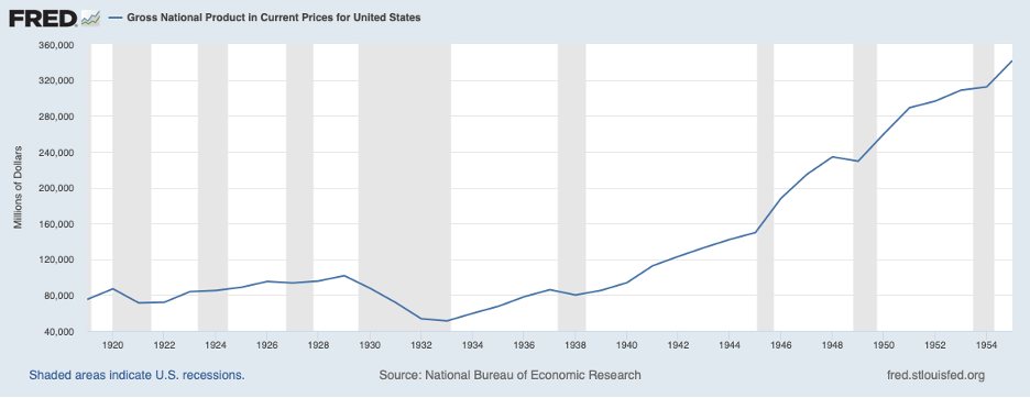
If we look at Gross National Product, we see that there was a big decline in the Great Depression, and nominal GDP doesn’t even return to 1929 levels until the 1940s. Then, it basically triples, from about $80 billion to about $240 billion. This was despite the large devaluation of the USD in 1933.
If we look at the “consumer price index” for the time, we see a big drop in the 1930s, and not much recovery until WWII. Then, it soars higher.
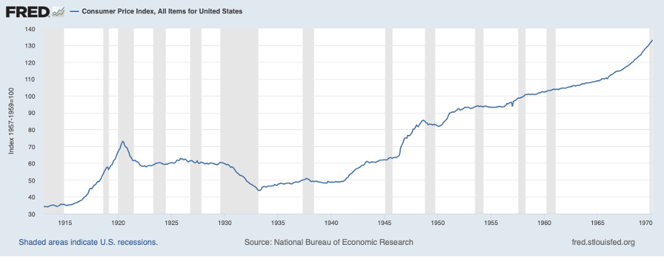
The modern CPI actually dates from a revision in 1940, and even then, was not much like today’s CPI. This is much closer to a broad commodities index. Nevertheless, it tells the basic story.
This CPI statistic was around 60 during the 1920s. In the 1950s, it was around 93. The devaluation of 1933 reduced the dollar’s value from $20.67/oz. to $35. This might be expected to cause a rise in prices of $35/$20.67, or 1.6933 (+69.33%), “all else being equal.” And indeed we find that 93/60 is +55%, right on target, and more accurate than we should have any expectation of seeing in real life, over such a long period, with such dubious statistics.
However, along the way, we see:
1) A big decline in the CPI due to recession in the early 1930s, accompanied by a decline in M2 and NGNP.
2) Stagnation in the CPI and also NGNP despite a large USD devaluation, due to a weak economy (and worsening economic policy).
3) A big expansion in the monetary base, M2, the CPI and NGNP during wartime due to “increased demand,” although there was not so much change in USD value during that time.
To summarize, there is indeed a correlation between M2 (bank lending), NGNP (the economy), and the CPI, although this often does not really reflect monetary conditions very well. Also, the way in which real monetary effects (the 1933 devaluation) play out in the economy is dependent on a variety of other factors.
This is also an interesting example — M2 for Japan:
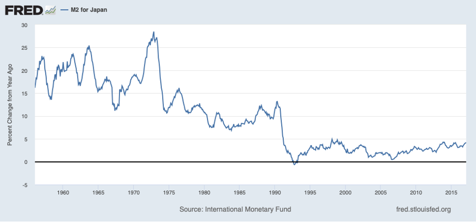
We see very high numbers in the 1960s, during the high growth era. There was no monetary inflation. The yen was linked to gold at 12,600 yen per oz. During the inflationary 1970s, M2 growth actually declined considerably.
Thus, we see that “M2” is certainly interesting, as a measure of bank lending activity, which his highly correlative and to some degree causative to economic activity as a whole, but doesn’t really have much relationship to monetary conditions. They may coincide, or they may not.
In general, I would say that being able to grasp these things is a sort of litmus test or rite of passage, that anyone aspiring to economic understanding has to pass before moving on to the more advanced levels. You can see that many don’t make it, and instead get stuck thinking that “M2,” or any other such “monetary aggregate,” has a significance that it really doesn’t have.
